Page 72: of Offshore Engineer Magazine (Oct/Nov 2014)

71 73

the results from the subsequent pigging operation with the difference in the amount removed believed to be due to solids left in the pipeline.

Pipelines

Avoiding pitfalls

The UT monitored locations were shown to have covered a good representation of where the highly corroded sections would be, although several other loca- tions were highlighted as potentially hav- ing a more corrosive environment. The work highlighted the potential pitfalls in using engineering judgment for inspec- tion purposes. But, although the locations were shown to be a good representation in this case, it could have been quite different. By inspecting the bathymetry

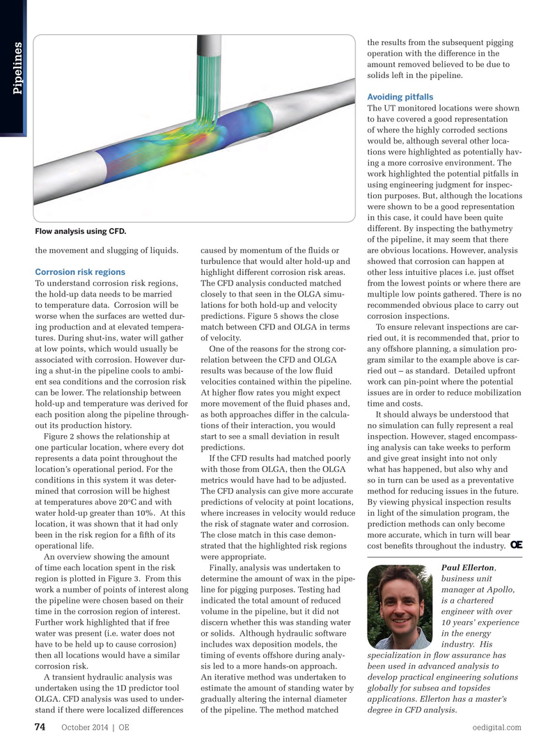
Flow analysis using CFD.

of the pipeline, it may seem that there the movem caused by momentum of the fuids or are obvious locations. However, analysis ent and slugging of liquids. turbulence that would alter hold-up and showed that corrosion can happen at

Corrosion risk regions highlight different corrosion risk areas. other less intuitive places i.e. just offset

To understand corrosion risk regions,

The CFD analysis conducted matched from the lowest points or where there are the hold-up data needs to be married closely to that seen in the OLGA simu- multiple low points gathered. There is no to temperature data. Corrosion will be lations for both hold-up and velocity recommended obvious place to carry out worse when the surfaces are wetted dur- predictions. Figure 5 shows the close corrosion inspections. ing production and at elevated tempera- match between CFD and OLGA in terms To ensure relevant inspections are car- tures. During shut-ins, water will gather of velocity. ried out, it is recommended that, prior to at low points, which would usually be One of the reasons for the strong cor- any offshore planning, a simulation pro- associated with corrosion. However dur- relation between the CFD and OLGA gram similar to the example above is car- ing a shut-in the pipeline cools to ambi- results was because of the low fuid ried out – as standard. Detailed upfront ent sea conditions and the corrosion risk velocities contained within the pipeline. work can pin-point where the potential can be lower. The relationship between At higher fow rates you might expect issues are in order to reduce mobilization hold-up and temperature was derived for more movement of the fuid phases and, time and costs.

each position along the pipeline through- as both approaches differ in the calcula- It should always be understood that out its production history. tions of their interaction, you would no simulation can fully represent a real

Figure 2 shows the relationship at start to see a small deviation in result inspection. However, staged encompass- one particular location, where every dot predictions. ing analysis can take weeks to perform represents a data point throughout the If the CFD results had matched poorly and give great insight into not only location’s operational period. For the with those from OLGA, then the OLGA what has happened, but also why and conditions in this system it was deter- metrics would have had to be adjusted. so in turn can be used as a preventative mined that corrosion will be highest The CFD analysis can give more accurate method for reducing issues in the future. at temperatures above 20°C and with predictions of velocity at point locations, By viewing physical inspection results water hold-up greater than 10%. At this where increases in velocity would reduce in light of the simulation program, the location, it was shown that it had only the risk of stagnate water and corrosion. prediction methods can only become been in the risk region for a ffth of its The close match in this case demon- more accurate, which in turn will bear operational life. strated that the highlighted risk regions cost benefts throughout the industry.

An overview showing the amount were appropriate.

Paul Ellerton, of time each location spent in the risk Finally, analysis was undertaken to business unit region is plotted in Figure 3. From this determine the amount of wax in the pipe- manager at Apollo, work a number of points of interest along line for pigging purposes. Testing had is a chartered the pipeline were chosen based on their indicated the total amount of reduced engineer with over time in the corrosion region of interest. volume in the pipeline, but it did not 10 years’ experience

Further work highlighted that if free discern whether this was standing water in the energy water was present (i.e. water does not or solids. Although hydraulic software industry.  His have to be held up to cause corrosion) includes wax deposition models, the specialization in fow assurance has then all locations would have a similar timing of events offshore during analy- been used in advanced analysis to corrosion risk. sis led to a more hands-on approach. develop practical engineering solutions

A transient hydraulic analysis was An iterative method was undertaken to globally for subsea and topsides undertaken using the 1D predictor tool estimate the amount of standing water by applications. Ellerton has a master’s

OLGA. CFD analysis was used to under- gradually altering the internal diameter degree in CFD analysis.

stand if there were localized differences of the pipeline. The method matched

October 2014 | OE oedigital.com 74 000_OE1014_Pipelines3_Apollo.indd 74 9/23/14 6:48 PM